Credit value adjustments (CVAs) are a key aspect of financial reporting and also Basel capital requirements for banks. The calculation of CVA is complex with difficultly around the parameterisation, modelling and technology infrastructure.

This blog aims to help you understand the main mechanics behind CVAs, credit exposure and default probability calculations, as well as provide an overview of wrong-way risk.

Exposure

The main defining characteristic of credit exposure (hereafter referred to as exposure) is whether the effective value of the contracts – including collateral – is in a party’s favour, positive, or against them – negative.

This is illustrated in Figure 1:

•  
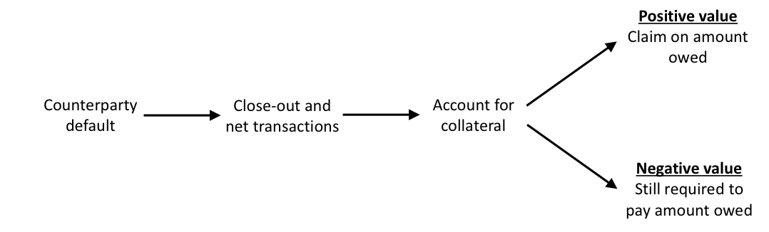
• Negative value – In this case, the party is in debt to its counterparty and is still legally obliged to settle this amount. A party does not[1] generally gain or lose from their counterparty’s default.
• Positive value – When a counterparty defaults, they will be unable to undertake future commitments, and thus a surviving party will have a claim – typically as an unsecured creditor. They will then expect to recover some fraction of their claim, just as bondholders receive some recovery of the face value of a bond.

Figure 1 Illustration of the impact of a positive or negative value in the event of the default of a counterparty.

We can define exposure as:

The amount represented by the “value” above represents the actual value of the relevant contracts at the default time of the counterparty. The value includes the impact of risk mitigants such as netting and collateral in line with contractual terms. Due to the difficulties around the close-out process, this is impossible to model precisely but the base value (i.e. with no valuation adjustments) is generally used as a proxy.

The exposure can also be seen as similar to an option payoff. This means that volatility is an important component and that, like pricing options on derivatives, exposure quantification is a difficult task.

Quantifying exposure is extremely complex due to the many different market variables that may influence the exposure, risk mitigants such as netting and collateral, and the long periods involved (Figure 2).

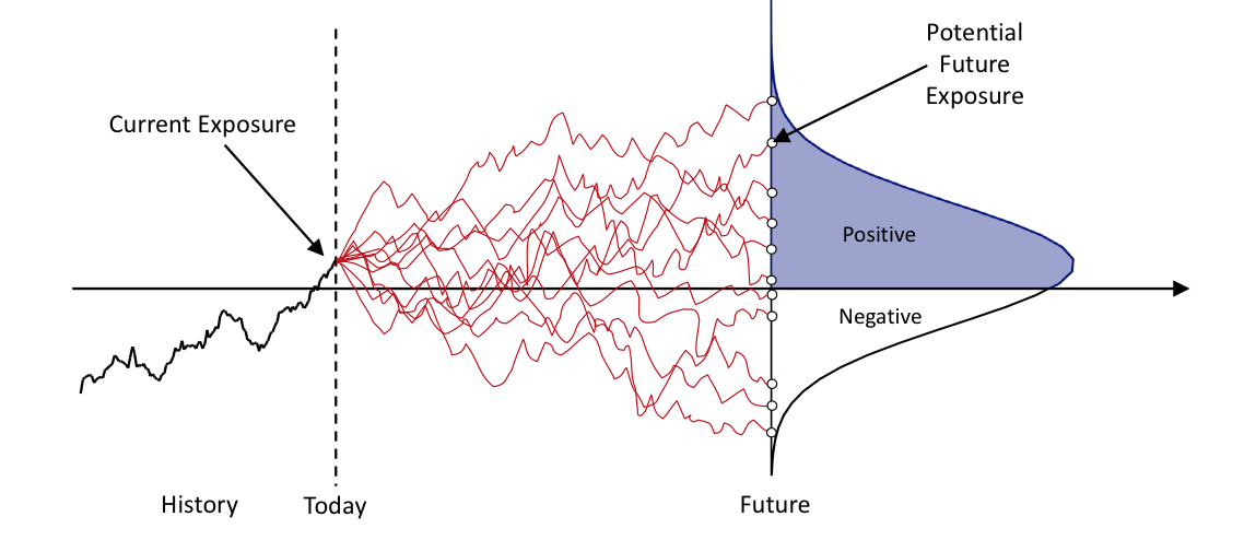
Figure 2. Illustration of quantifying future exposure.

There are several important metrics used when quantifying exposure which are all based on the distribution of future value (Figure 3):

• Expected future value (EFV) – This component represents the forward or expected value; it's the average over all scenarios.
•  
• Potential future exposure (PFE) – As discussed, PFE represents the largest exposure at a certain confidence level. PFE is a similar metric to value-at-risk (VAR).
•  
• Expected exposure (EPE) – EPE is the average of all positive exposure values. Note that only positive values give rise to exposures which means that the EPE is above the EFV. Note that EPE is sometimes called expected exposure (EE).
•  
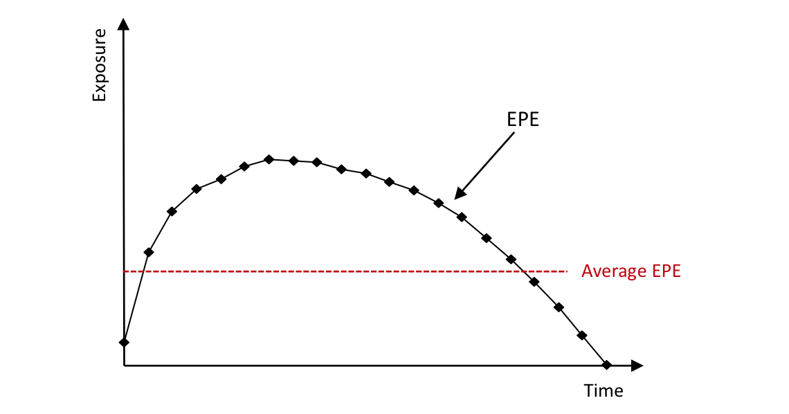
• Average EPE – This is defined as the average exposure across all time horizons and is therefore the (weighted) average of the EPE across time (Figure 4). This single number is often called a “loan equivalent”, and is the average amount effectively lent to the counterparty.

Figure 3. Illustration of exposure metrics for a single time horizon.

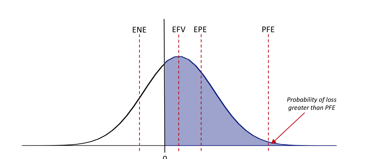
Figure 4. Illustration of EPE over time and the average EPE.

Exposure is represented by positive future values. Conversely, we may define negative exposure as being represented by negative future values. This will represent the exposure from a counterparty’s point of view. We can define measures such as expected negative exposure (ENE) which are important when computing metrics such as DVA and FVA.

Default Probability

There are typically two types of default probability; real-world and risk-neutral. A real-world default probability is often estimated from historical default data via some associated credit rating. A risk-neutral default probability is taken from market prices such as CDSs. Investors require an embedded premium when taking credit risk, so risk-neutral default probabilities are generally larger than real-world probabilities (Figure 5).

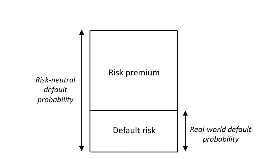
Figure 5. Illustration of the difference between real-world and risk-neutral default probabilities.

One empirical example showing the difference between real-world and risk-neutral default probabilities is shown in Table 1. The differences are large, especially for strong quality credits.

Table 1. Comparison between real-world and risk-neutral default probabilities in basis points. Source: Hull et al (2005)[2].

In the past, it was common for banks to use real-world default probabilities (based on historical estimates) to quantify CVA. Now, it's standard for risk-neutral default probabilities to be used. This move has been catalysed by accounting requirements and Basel III capital rules and regulations in general.

For example, EBA (2015)[3] states:

“The CVA data collection exercise has highlighted increased convergence in banks’ practices concerning CVA. Banks seem to have progressively converged in reflecting the cost of the credit risk of their counterparties in the fair value of derivatives using market implied data based on CDS spreads and proxy spreads in the vast majority of cases. This convergence is the result of industry practice, as well as a consequence of the implementation in the EU of IFRS 13 and the Basel CVA framework.”

Some smaller and regional banks still use real-world default probabilities and justify this with arguments that they have no credit spread data with which to benchmark parameters and that this conforms to the practice in their region. However, this position has become increasingly untenable in recent years.

Since many counterparties do not trade in the CDS market, risk-neutral default probabilities need to be defined via relevant proxies. This is typically done with mapping based on the rating, region and sector of the counterparty in question. Liquid credit spread information from single-name CDS, index CDS and other traded credit spreads are used.

Assuming the relevant spread can be calculated then a common approximate formula for risk-neutral default probabilities is:

Where the default probability is up to is the credit spread at the time and is the assumed loss given default.

Calculating CVA

The standard formula for CVA is:

CVA depends on the following components:

• Loss given default (LGD) – the percentage amount of the exposure expected to be lost if the counterparty defaults.
•  
• Expected exposure (EPE) – the discounted expected positive exposure (EPE) for the relevant dates in the future (Section 1.1).
•  
• Default probability (PD) – requires the default probability which can be calculated via equation (3).

There is also a quicker way to estimate the above result that's useful for simple calculations. This formula assumes that the EPE is constant over time and equal to its average value which yields the following approximation:

Where the CVA is expressed in the same units as the credit spread, which should be for the maturity of the instrument in question, and EPE is as defined in Section 1.1.

Wrong-way Risk

In the quantification of CVA, wrong-way risk (WWR) is sometimes ignored as in Equation (3) above (due to the default probability and EPE being treated independently and simply multiplied together). WWR is the phrase generally used to show an unfavourable dependence between exposure and counterparty credit quality: the exposure is high when the counterparty is more likely to default which will increase CVA. WWR is difficult to identify, model and hedge due to the often subtle macro-economic and structural effects that cause it.

One classic example of WWR is a cross-currency swap where a potential weakening of the currency and simultaneous deterioration in the credit quality of the counterparty is dangerous. This would be the case in trading with a sovereign and paying their local currency – or more likely, in practice, hedging this trade with a bank in that same region. Alternatively, the default of a sovereign, financial institution, or large corporate counterparty may precipitate a currency weakening.

Although it may often be a reasonable assumption to ignore WWR, its manifestation can be potentially dramatic. In contrast, right-way risk can exist in cases where the dependence between exposure and credit quality is a favourable one. Right-way situations will reduce counterparty risk and CVA. Regulators have identified both general (driven by macro-economic relationships) and specific (driven by causal linkages between the exposure/collateral and default of the counterparty) WWRs as critical to measure and control.

Beyond CVA

The starting point

Pricing derivatives has always been relatively complex. However, before the global financial crisis, the pricing of vanilla products was understood and most attention was on so-called exotics. Credit, funding and liquidity were ignored since their effects were viewed as negligible.

This old-style framework has undergone a revolution to address the shortcomings highlighted by the crisis and properly incorporate aspects such as funding and collateral agreements. Nowadays, derivatives contracts tend to be quite simple (very few exotics) but they are valued and managed in a more sophisticated framework.

One change has been the move away from the use of LIBOR to discount future cash flows. For many years, LIBOR was seen as a good proxy for the risk-free rate. Now the OIS (overnight indexed swap) is seen as the most obvious risk-free rate and can be shown to be the correct discount rate for a “perfectly collateralised transaction”.

Perfect collateralisation means that the amount of collateral held or posted will be, at all times, identical to the positive or negative value of the transaction and denominated in the same currency. Although this is never perfectly achieved in practice, it's a reasonable starting point and some transactions are considered by the industry to be close to this theoretical ideal, notably:

• centrally cleared trades - from the CCP point of view; and interbank trades – due to collateral agreements with zero thresholds and daily collateral posting.

So OIS discounting can be seen as a base case and xVA components can then be added/subtracted as relevant.

The Birth of xVA

In the aftermath of the global financial crisis, CVA attracted huge interest due to the problems associated with counterparty risk, the reaction of regulators with the Basel III CVA capital charge, and accounting changes with IFRS 13. However, as part of these changes, other aspects connected to CVA started to gain considerable interest. The xVA terms arise from assessing rigorously the lifetime cost of an OTC derivative, including all economically relevant terms as illustrated in Figure 6. The explanation of the different aspects is as follows:

• Positive value – When the transaction (or portfolio) has a positive value – above the centre line – then the uncollateralised component gives rise to counterparty risk and funding costs. If some or all of the value is collateralised, then the counterparty can choose what type of collateral to post.
•  
• Negative value – When the transaction has a negative value then there is a counterparty risk benefit from the party’s own default and a funding benefit to the extent their counterparty is uncollateralised. If collateral is posted, then the party can choose the type to post.
•  
• Overall – Whether or not the transaction has a positive or negative value, there are costs from the capital that must be held against the transaction and any initial margin that needs to be posted.

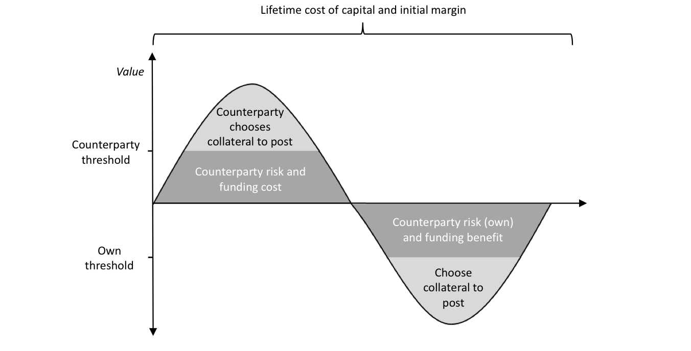
Figure 6. Illustration of the lifetime cost of an OTC derivative. Note that this representation is general, and in reality, thresholds are often zero or infinity.

Computing xVA

The general concept of any xVA term is illustrated in Figure 7. This quantifies the value of a component such as a counterparty risk, collateral, funding or capital. Generally, the terms are associated with a cost but note that in some cases they can be benefits. To compute xVA we have to integrate the profile shown against the relevant cost or benefit such as a credit spread, collateral, funding or cost of capital metric.

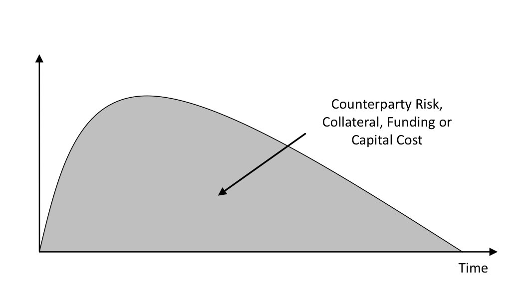
Figure 7. Generic illustration of an xVA term. Note that some xVA terms represent benefits and not costs and would appear on the negative y-axis.

Calculating xVA involves integrating the relevant profile against the underlying cost or benefit such as a credit spread, collateral, funding or cost of capital metric. The quantification of the profile itself is generally a significant quantification challenge with issues over model choice, calibration and numerical tractability. In general, it requires the valuation of option-like payoffs. However, in certain cases, the valuation collapses to essentially pricing forward contracts and is, therefore, largely model-independent. These special cases can be dealt with by changing discounting assumptions. There is also the problem of defining the cost component – credit spreads and funding, collateral and capital costs – which is a difficult qualitative problem.

xVA Terms

Assuming, we start from a basic valuation such as OIS discounting, there are a variety of xVA terms defined as follows to achieve the correct valuation (Figure 8):

• CVA and DVA – Defines the bilateral valuation of counterparty risk. DVA (debt value adjustment) represents counterparty risk from the point of view of a party’s own default.
•  
• FVA – Defines the cost and benefit arising from the funding of the transaction.
•  
• ColVA – Defines the costs and benefits from embedded optionality in the collateral agreement – such as the ability to choose the currency or type of collateral to post – and any other non-standard collateral terms compared to the idealised starting point.
•  
• KVA – Defines the cost of holding capital – typically regulatory – over the lifetime of the transaction.
•  
• MVA – Defines the cost of posting initial margin over the lifetime of the transaction.

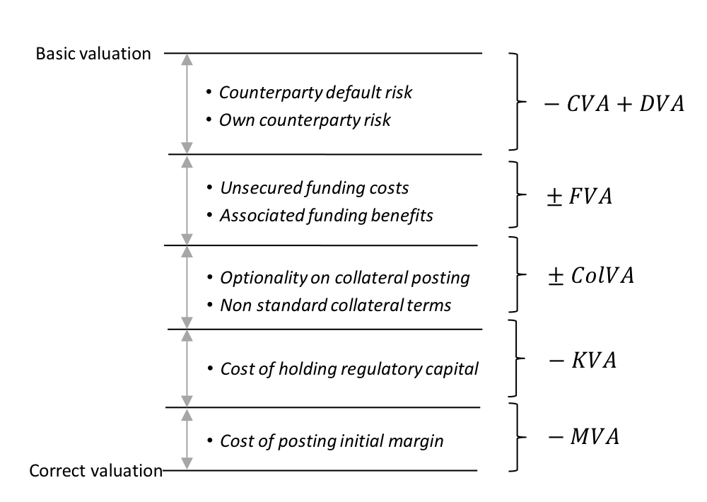
Figure 8. Illustration of the role of xVA adjustments.

It is also important to note that there are potential overlaps between the above terms. For example, between DVA and FVA where own default risk is widely seen as a funding benefit.

Knowing how to calculate your default probability and credit exposure can help you determine if a credit or position is financially worthwhile for your portfolio; you’ll be able to see how much risk you’re assuming by accepting a certain trade or position, and whether or not it will increase volatility in your portfolio.

If you want to learn more about CVAs and counterparty risk, contact us today to get access to a specialist course on this topic. We work solely with world-class financial experts to bring you cutting-edge courses that can answer any questions you may have.

Related Courses

Bilateral Margining and Central Clearing

Valuation Adjustments: The XVA Challenge

^[1] This is not completely true due to the complexity of the close-out process.

^[2] Hull, J., M. Predescu, and A. White, 2005, “Bond Prices, Default Probabilities and Risk Premiums”, Journal of Credit Risk, Vol. 1, No. 2 (Spring), pp. 53-60.

^[3] European Banking Authority (EBA), 2015, “On Credit Valuation Adjustment (CVA) under Article 456(2) of Regulation (EU) No 575/2013 (Capital Requirements Regulation - CRR)”, February, www.eba.europe.eu.