This article was first published in the Journal of Performance Measurement Volume 27-4, Summer 2023
Part 1 of this article was the first known attempt to categorise and compare across implemented FIA models using a common dataset.
The objective was to see if a ‘Generic’ Model could be defined for FIA in the same way that Brinson has become one for Equity Attribution.
No ‘Generic Model’ exists for Fixed Income Attribution. Instead, different academics working alone or with software suppliers have, historically, individually designed models.
Part 1 identified significant commonality as well as differences across the four models compared. Two years on, Part 2 adds a further three models to the analysis, seeking through the increased number to confirm the Part 1 commonality identified and, with the passage of time, detect any new commonality and/or reporting trends.
INTRODUCTION
Until release of the 2020 Performance Standards, GIPS compliance restricted Firms to the Modified Dietz/Time Weighted algorithm for Performance Reporting. The 2020 flexibility, section 1.A.35, additionally allowed Money Weighted returns where firms have control of external cash flows.
Whilst not part of GIPS, Equity Attribution enjoys near-global algorithm standardisation via Brinson Additive. Significant flexibility has, however, arrived since its 1985 introduction. The ‘Bottom Up’ alternative to the original ‘Top Down’ approach is one example. We also see the optional geometric algorithms, different approaches to the treatment of non-Benchmark securities and different multi-period smoothing options.
Fixed Income Attribution, with us now for over 30 years, offers near-total flexibility, being viewed as a series of independent models lacking standards or even, apparently, commonality. Accordingly, FIA implementations, recently termed a ‘non standardised endeavour’ (Aite-Novarica, 2021), offer significant configurability in order to meet user requirements, see further below.
Part 1 of this article considered the options for greater standardisation via a Brison-like ‘Generic Model’. As the first stage in such a journey it sought cross-model commonality.
Part 1’s method was to calculate and compare the returns produced by different models from a single set of data. This journal’s FIA model articles to date and the model descriptions in the Public Domain have used independent data sets thus complicating direct comparison of commonality.
Part 1 scope included the:
- (a) selection of four models on the basis of their returns/algorithms being in the public domain
- (b) calculation and comparison of returns for all four from a common set of investment positions and market data (Q1 2020, which also highlights a ‘flight to quality’)
- (c) returns calculated as portfolio contribution/fund level only for three of the models, active return/sector level for the fourth
- (d) instrument type Foreign Corporate Bonds to give the maximum number of potential returns
- (e) output treated as ‘indicative’ given that the market data was historic, part incomplete and returns were not being calculated by the model authors.
Commonality was identified across all four models in the ‘Income’ and ‘Price’ (ie Government + Corporate Term Structures) return categories even though the levels of analysis and the algorithms employed under each of these varied. Income Return, for example, was defined by different models as any of Current Yield, Yield to Maturity and Accrued Income Yield. Existence of other return categories, for example Currency, Swap Curve, Instrument Specific, varied by model.
Part 1 also identified the existence of three FIA categories - ‘Bottom Up’, ‘Top Down’ and ‘Hybrid’. The models compared offered anything from one to all three of these approaches, the ‘Hybrid’ case comprising two separate reports, each independently reconciling to the Active Return.
PART 2 – INITATIVE
Post Part 1, consideration was given to enhancing its observations via further model coverage.
This required:
- (a) the identification of further models/software suppliers
- (b) the availability of model details/algorithms available in the Public Domain, or
- (c) the cooperation of model authors/software developers.
Aite-Novarica’s 2021 ‘FIA best in class Matrix’ publication was used as the start point for (a). Of the thirteen models/suppliers listed in the Matrix, two had already been covered in Part 1. Of the remainder, ten of the suppliers were contacted with view to participation in Part 2. Of these, three kindly agreed to become involved in the production of returns from the same Part 1 dataset, for which the author is most grateful. Some calculated returns themselves, others provided algorithms.
Whilst not the most statistical approach to selection, it has proved useful all the same.
PART 2 – APPROACH
Data
The following dataset enhancements were introduced for Part 2:
- (a) a benchmark was added to provide benchmark-relative reporting across all models. For simplicity, the benchmark securities are the same as the portfolio positions and meaningful active returns have been achieved by varying the portfolio/benchmark weightings
- (b) sector level returns were enabled for all models
- (c) Security level reporting was added where relevant.
Models Compared
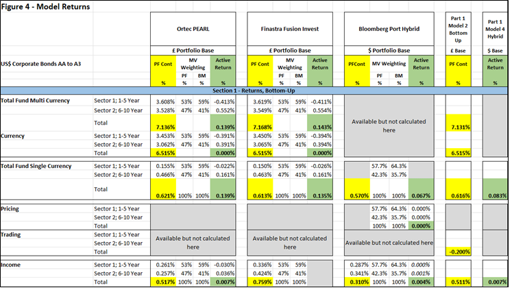
The returns of the three new models were compared to each other and to those of the two most relevant Part 1 models (Figure 4). The chosen Part 1 models were the ‘Extended Bottom Up’ (£ base) and Flametree Hybrid (US$ base).
Model Categories
The model categories identified in Part 1, Bottom-Up (BU), Top-Down (TD) and Hybrid (ie includes both BU and TD characteristics) persist in Part 2 although an alternative definition of Hybrid also became apparent.
The following similarities/differences in comparison to Brinson/Equity Attribution, from which the TU, BU and Hybrid terms have been adopted, were identified:
Similarities
- BU; as with the Bottom-Up management of Equity Funds this approach reflects primacy of lower ie security-level decisions subsequently aggregating up to sector/portfolio totals.
- TD; reflects the higher, sector allocation decisions being primary ie which currencies, sectors and what duration positioning.
Differences
- Portfolio Contribution, Active Return or both? Both are valid FIA/BU start points. Whilst Brinson by definition is purely benchmark-relative, FIA/BU/Portfolio Contribution is useful in itself in providing information on the sources of return.
TD, however, is always benchmark-relative.
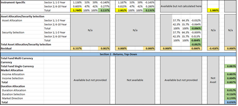
- Brinson for FIA? Whilst the classic Brinson Returns of Asset Allocation and Stock Selection were initially considered to be too minor a contributor to FIA to be included, as models developed it made a TD ‘comeback’. Part 1 showed Income Return to be restated under TD as an AA/SS returns (slightly ironically, as excluding ‘Interaction’ is a ‘Bottom-Up Brinson’ approach) and an extension of this appears in Part 2.
Model Configuration
FIA’s quoted ‘non-standard endeavour’ partly provides the flexibility required to meet varying user requirements within the complex discipline of Fixed Income Funds Management.
FIA moves away from the limited flexibility applying to Performance Reporting/Equity Attribution systems, reasons including the following:
- (a) Equity Attribution almost always reports at sector level. Although sectors are user defined (eg normally industry but also, say, country) the concept is straightforward. The rough FIA sector equivalent of ‘Yield Curves’ is a far larger concept, potentially embracing Swap, Corporate, Issuer and Country Curve Types. A Curve is a combination of available market data and supplier static data. Each has a ‘Yield Spread’ vs the ‘Risk Free’ or Treasury Curve from which returns can be calculated. Depending on fund type and user requirement some or all of these Curves may be required resulting in suppliers offering multiple models
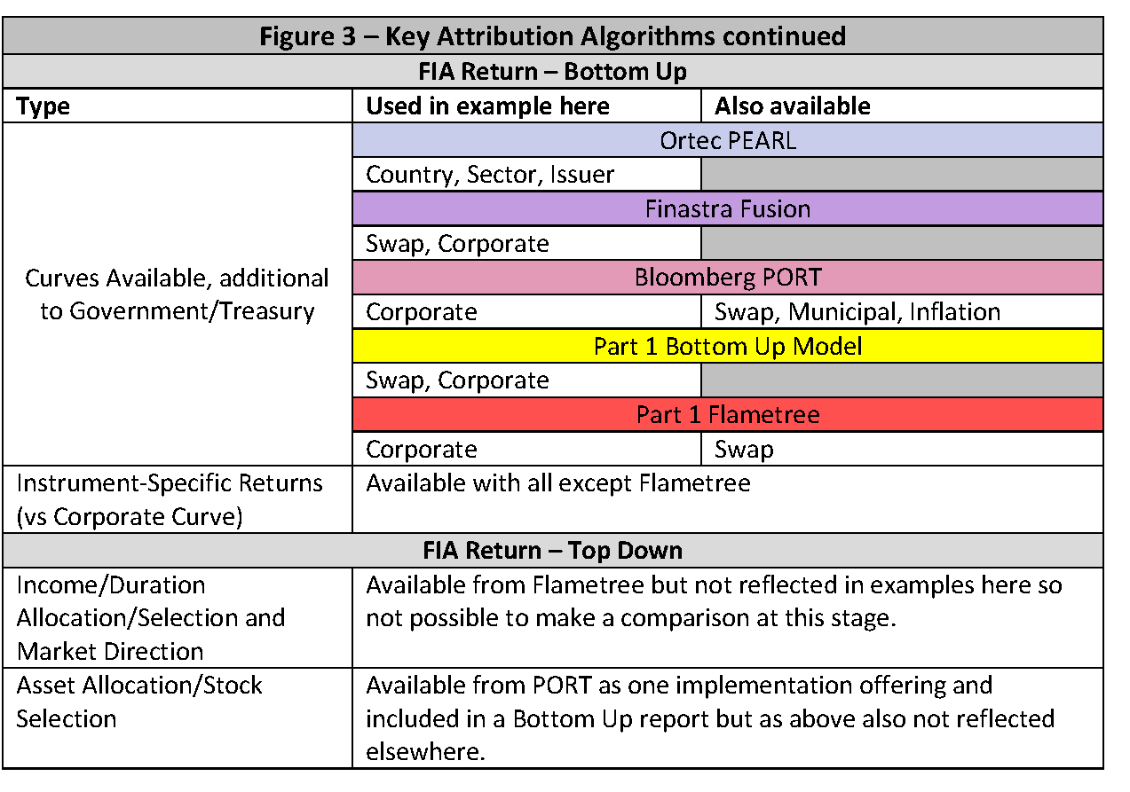
- (b) User requirements may determine the reporting of individual instruments’ returns vs ‘their own Curve’, a form of Selection Return unique to FIA
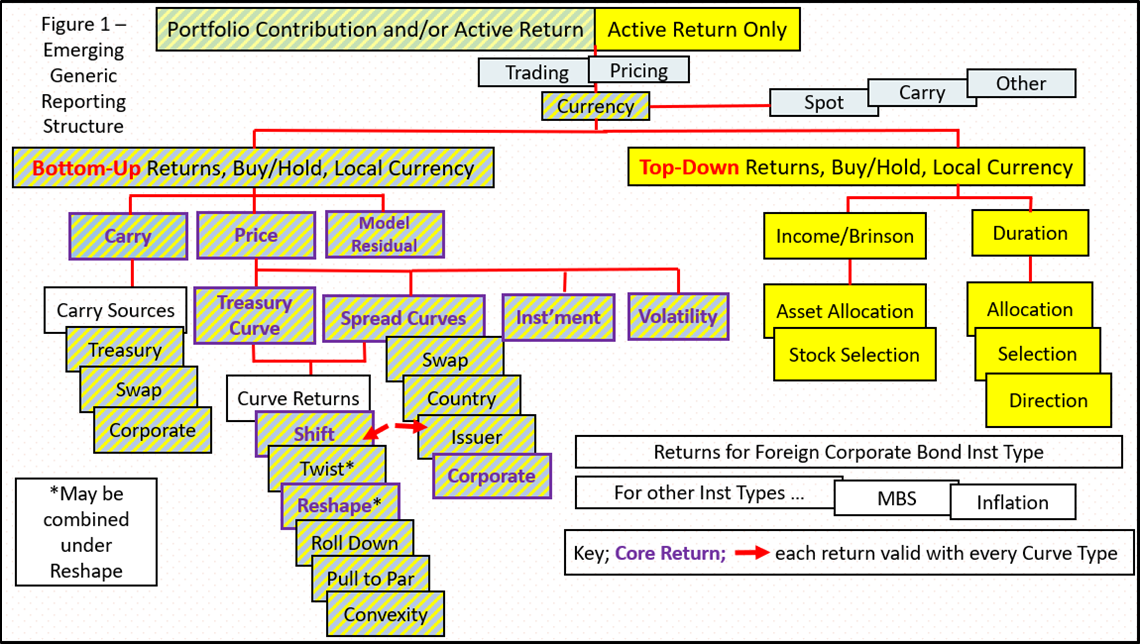
- (c) Within each Curve a variety of returns potentially apply; Figure 1 listing six across five Curve Types giving a potential maximum thirty returns
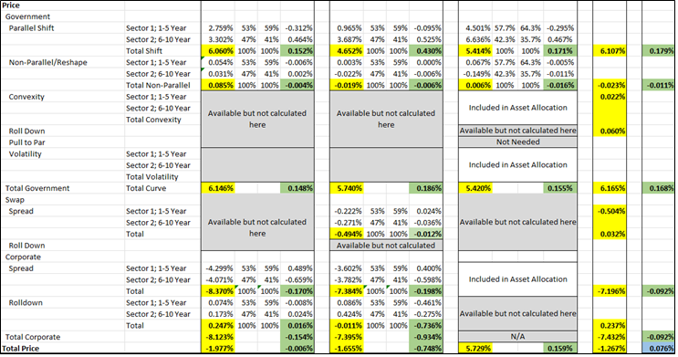
- (d) Returns from the Government Curve potentially arise from ‘Parallel Shift’, ‘Twist’ and/or ‘Other’ Yield Curve movements as well as Curve Rolldown. With the Corporate Curve the same apply to the ‘Spread Return’
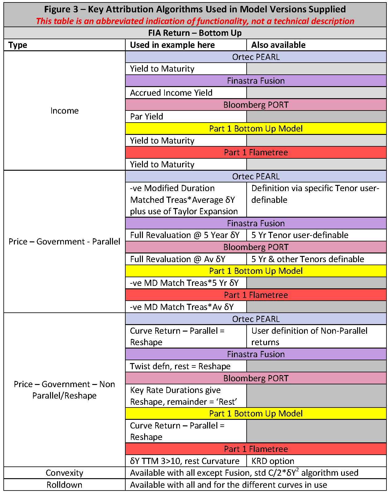
- (e) Curve Returns can be calculated via the ‘short cut’ method of multiplying yield change by the -ve of Modified Duration plus perhaps adding Convexity or by the lengthier process of Full Revaluation. Again, there is no standardisation here, both methods appearing across the five models compared (Figure 4)
- (f) ‘Model Residual Return’ – something Brinson users have sought for decades to eliminate(!) – has validity as we are comparing Mark to Market to Mark to Model. Accordingly some explicit Residual will always appear unless ‘hidden’ within a ‘difference’ return.
This complexity of approach means that returns (Figure 4) will not exactly reconcile across models.
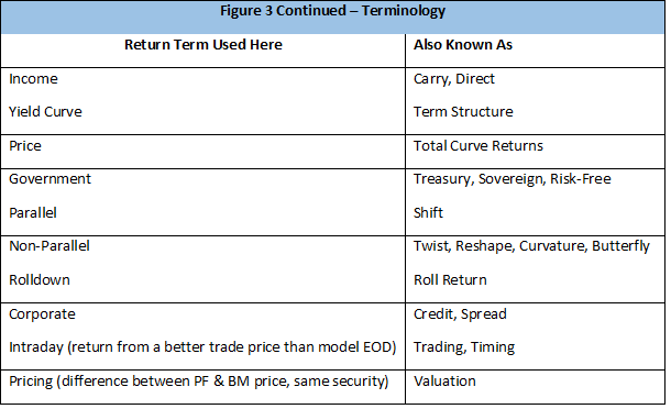
Comparing Government Curve Parallel Return, for example. Figure 3 shows that some model versions used have based this on 5-year Tenor δY, others on Curve Average δY (choice often configurable). This will give return differences. Further, with data, the practical result of analysing the Part 1 Portfolio – level returns into Part 2 Sector-level returns has introduced small differences.
With production, some of the returns have been produced via the daily calculations of the systems themselves, others as a single quarterly spreadsheet-based return. This also will give small variations in returns.
Given this, a number of the cross-model returns in Figure 4 are remarkably close, giving support to theory of commonality.
Aside from specific returns, the Figure 4 output usefully shows the Return Categories available across all models, both Core (all models) and Non-Core (some models only) Returns.
PART 2 – OUTPUT SPECIFICS
Return Mechanics
The first reporting step is to confirm the Performance Return (Portfolio Contribution or Active Return) start point.
BU attribution calculations normally follow next with TD attribution where offered as the last step.
Return Algorithms
Figure 3 below gives an indication of the algorithms used across models in both Parts 1 and 2.
Commonality/Bottom Up and Top Down
Considerable commonality persists across BU, especially across the ‘Core Returns’ of Part 1.
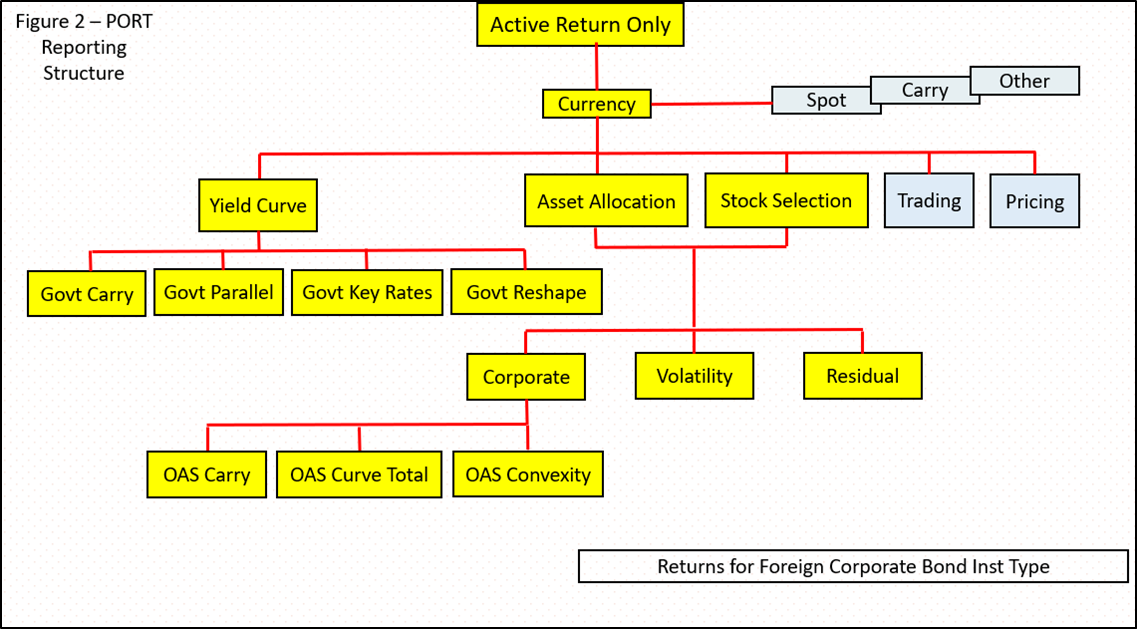
With TD, the ‘Full Hybrid’ Flametree model of Part 1 wasn’t replicated by the Part 2 models. It doesn’t mean Full Hybrid lacks validity, just that the relevant (different) models were not offered as part of Part 2. For example, while the particular Bloomberg PORT model used showed a different Hybrid approach (a combined set of BU/TD returns, Figure 2), this was only one model option and other model types exist which can replicate the Flametree approach.
Sector Weightings/Instrument Classifications
Figure 4 shows common Portfolio and Benchmark Sector Weightings across four of the five models. The slightly different Bloomberg PORT weightings arise because one security qualified for a shorter TTM during the reporting period and the system correctly reflected that.
Instrument Configuration
For instrument types beyond bonds, Fusion Invest, for example, offers a pricing library and toolbox, allowing managers to user-define valuations and FIA return.
CONCLUSIONS
Bearing in mind the limited number of models compared thus far across both Parts of this article:
- (a) the FIA BU, TD and Hybrid concepts persist while recognising user configurability around this
- (b) the BU models show the beginnings of a ‘Generic’ reporting approach, especially with the ‘Core’ returns (Figure 1)
- (c) the limited output available at this stage makes it difficult to make the same conclusions for TD or Hybrid, although Part1/TD structure is included in Figure 1 for information
- (d) the different return algorithms used across models indicate that, although returns can be close, algorithm standardisation is distant.
References
‘Aite Matrix: Fixed Income Attribution and Analytics’ Paul Sinthunont and Audrey Blatter, Aite-Novarica, April 2021
‘Decision Driven Fixed Income Attribution’ Pam Zhong, October 2012
I am most grateful to Bas Leerink of Ortec Finance and to Fabien Trigano of Finastra Fusion for their assistance with this article and to Ian Thompson, Carl Bacon and Tim Escott for their peer reviews and general assistance. Any errors remain entirely my own responsibility.
To learn more about Fixed Income Attribution from world-leading practitioners, register for our Fixed Income Attribution course.