Finance101 teaches us that a dollar next year is worth less than a dollar today. Formally, we write for the present value of a promised, or expected, cashflow CT :

… where the discount factor is given by:

What Finance101 fails to discuss is what the rT represents. A common stance on fixed-income is that the discount rate is a credit-adjusted yield that reflects the creditworthiness of the bond. By contrast, derivatives textbooks, typically after some algebraic manipulations involving a binomial tree, assert that the PV of any derivative is the expectation value of the future cashflow evaluated in the risk-neutral measure discounted at the risk-free rate.
There are several problems with this:
- It directly contradicts what we learn in fixed-income
- Market practice for 30 years was to use LIBOR as the risk-free rate, which – as beleaguered owners of UK bank shares will attest – is nonsense.
On that note, I will aim to correct decades of inaccurate explanations and put the record straight by demonstrating: what the OIS Revolution was all about, where XVA adjustments come from, the crucial role of collateralisation and how the terms of the CSA drive the construction of a valuation curve.
We’ll work with continuously-compounded rates as a convenient fiction; it doesn’t affect any of the arguments.
Separating market risk from credit risk
Let’s start with a quiz. What is the flat discount rate appropriate for PV’ing the cashflows of:
- A 3-year UST - assumed to be risk-free for this exercise - yielding 2%?
- A 3-year corporate bond whose debt trades at T+100?
If you answered 2% or 3%, I’m afraid to say you’re wrong - not in practice, but in principle.
The mistake is to confuse discounting, a measure of market risk, with a default-risk adjustment which is a measure of credit risk. These risks are unrelated and should be priced and managed separately.
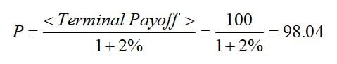
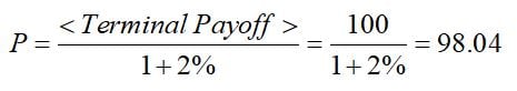
Take, for example, a 1-year risk-free zero-coupon bond where 1-year rates are 2%. The price is calculated as:
Now consider a 1-year zero-coupon bond issued by a struggling corporate with a 1% chance of defaulting in the next 12 months and no recovery value. The market risk – interest rate risk – of the position is identical, so we use the same discount rate, but the expected payoff at expiry is now only 99.
With this in mind, the right approach to pricing is:
Although this is the correct answer, it’s not what anyone in the bond world does. Instead, we perpetuate a colossal fudge, defining an incremental credit spread σ that happens to work, via:
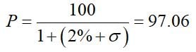
This tells us that σ = 1.03%, or we say the corporation is trading at ‘103 over Treasuries.’ [The close agreement between the stated default probability and the credit spread is not a coincidence – see the appendix].
Why it matters
So why is it important to separate market risk from credit risk? Can’t we just calibrate to credit spreads that happen to work and be done with it?
This approach fails because:
- Our model loses any predictive power, becoming useless for effective risk-management which is about forecasting and mitigating future risk.
- There is no single credit spread, or z-spread, even for a given maturity, so instead of having a single underlying parameter that captures credit risk we have a zoo.
- Most importantly – the approach doesn’t work for derivatives.
Let’s examine why. Consider a 1-year swap, analogous to the 1-year bond above, traded at the par rate of 2%, (versus LIBOR, for the sake of argument – it doesn’t matter), with an AAA counterparty.

Spot 12M LIBOR = 2% obviously, and this swap has PV = 0.
From the bank’s perspective:
PV Fixed -1.96078%
PV Floating +1.96078%
==========
Zero
However, if the counterparty is a B-rated corporate trading at 100 over, the swap would now be worth less. This is because there’s a non-zero probability of suffering a loss if the counterparty defaults while we have a positive MTM on the trade.
So how much is the swap worth? Following our calculation for the zero-coupon bond, we adjust our discount rate upwards by 100bp to reflect the credit impairment and get:
PV Fixed -1.94175%
PV Floating +1.94175%
==========
Still Zero!
This example demonstrates that pricing credit risk by the traditional method of shifting the discount curve simply doesn’t work, except for static, funded exposures such as bonds.
We need a new methodology to treat credit risk separately from market risk: this is where CVA will help you - its backwards-compatible approach works just as well for bonds and loans.
So we’ve established that the correct discount rate is a pure market risk number, completely decoupled from any counterparty risk considerations. In the next blog post, we’ll consider what that number should be.
Appendix – Default Risk and Credit Spreads
The standard model for default risk is to treat is a Poisson process with intensity λ; to be precise, the model assumes that the probability of default between t and t+dt, conditional on the company being alive at t, is given by:

With this definition it is easy to show that the probability of surviving to t is:

And therefore, the unconditional probability of a default between t and t+dt is:

Now consider the pricing of a T-year bond playing a coupon c (that is, in our continuous-time approximation a bond pays a cash amount of cdt in an interval dt), and will recover an amount R in the event of default.
The price of this bond, using a flat discount yield of r, is simply:
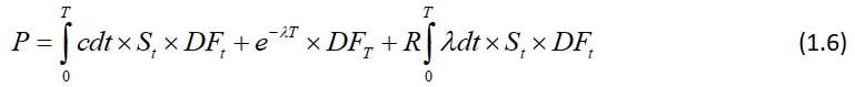
Which evaluates to:

Where I have defined the PV of an annuity  , and an asterisk represents a mapping r → r + λ.
There are two important observations to make about formula 1.7
- On the assumption of zero recovery, the pricing of default-risky debt is correctly done by mimicking the pricing of risk-free debt, with a simple incremental shift to the discount curve – the credit spread. The credit spread is equal to the hazard rate (the conditional default intensity).
- In a world with non-zero recovery, the shift-the-discount-curve approach – the z-spread approach – is inconsistent with the market’s standard model of default risk pricing, and therefore, assuming we would aim to hedge credit risk with CDS, is essentially useless.
Related Courses
Interest Rate Derivatives and SwapsInterest Rate Derivatives 2: Options
Interest Rate Derivatives 3: Structuring