In this article, we discuss:

• important and specific characteristics of default risk and methodological implications.
• how joint default probabilities might be a hidden source of risk in conventional portfolio models of default.

In their latest report, the OECD summarised corporate credit risk as:

“By the end of 2019, the global outstanding stock of non-financial corporate bonds reached an all-time high of USD 13.5 trillion in real terms. This record amount is the result of an unprecedented build-up in corporate bond debt since 2008 and a further USD 2.1 trillion in borrowing by non-financial companies during 2019, in the wake of a return to more expansionary monetary policies early in the year. The new data in this report shows that, in comparison with previous credit cycles, today's stock of outstanding corporate bonds has lower overall rating quality, higher payback requirements, longer maturities and inferior investor protection.

“While the growing stock of the BBB rated bonds has allowed investors to seek higher yields, their choice of portfolio allocation is typically influenced by regulations and defined by rating-based investment mandates. Given these limitations, together with a concentration of outstanding bonds just above the demarcation line between investment and non-investment grade, extensive downgrades of BBB rated bonds to non-investment grade status may lead to substantial sell-offs that put corporate bond markets in general under stress, giving rise to financial stability concerns.”

Extensive downgrades and sell-offs will affect investor portfolios in several ways, two of which are:

1. Increase of default risk for hold-to-maturity corporate credit exposure
2. Negative returns in corporate debt exposures which are marked-to-market (credit spread risk)

In addition to corporate debt, public debt had been increasing globally – a trend now accelerated by the coronavirus pandemic. Of course, the megatrend of ‘increasing debt’ is little more than the mirror image of the ‘low-interest rates’ and ‘low yield’ megatrend. The two trends interact, as investors – subject to target returns – are forced to take on more risk to earn the required yields on investments.

Rising credit risk exposures place an increasing focus on credit risk management techniques and analytics in investment portfolios. Credit risk differs in important aspects from market risk, which is at the centre of portfolio risk management in Modern Portfolio Theory. Unfortunately, a consensus among academics and researchers in credit risk management approaches does not exist.

The situation is further complicated by the fact that many credit risk measurement tasks and analytics are delegated to external credit rating agencies using their known, proprietary methodologies. This coexistence of competing approaches creates significant amounts of model risk in practical applications - in addition to the actual default risks in the investment portfolios.

In this article, we’ll show significant and specific characteristics of default risk and methodological implications and demonstrate that joint default probabilities might be a hidden source of risk in conventional portfolio models of default.

Default and Joint Defaults

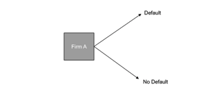
For analytical purposes, default can be defined as a two-state variable for a firm A: ‘in-default’ versus ‘not-in-default’. This can be visualized as follows:

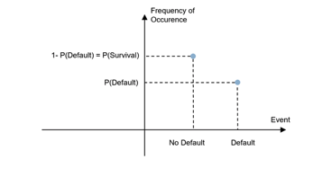
If we assume that the process of going from one state to another is not deterministic, such a binary variable turns into what is known as a Bernoulli distribution: a stochastic variable with two possible values realised with a certain probability. In our context, this probability is the default probability P. The histogram or probability distribution function of a Bernoulli variable is:

By introducing a second Bernoulli variable with the same probability, the possible outcomes increase from two to three: no default, one default, two defaults. Generally, n Bernoulli distributions define what is called a Binomial distribution. For two firms A and B, with differing default distributions p_A and p_B, the default probabilities and losses are defined as follows:

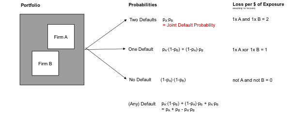
Joint defaults are a stress scenario because losses are cumulative and significant, potentially threatening the operation - or even continuation - of an investment portfolio.

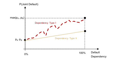
It is crucial to understand that binomial distributions of default work with a zero default dependency assumption, i.e. ‘zero default correlation’. Only under this assumption is the joint default probability equal to the product of the default probabilities of the firms. Unfortunately, this assumption does not conform to stylized facts about defaults, which are about clusters of defaults, factors affecting particular groups of creditors, or debt markets overall. For real-world illustrations, see the Financial Crisis of 2008; the OECD outlook also contains expectations of clustered credit downgrades and systemic effects.

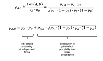
The joint probability of default, given independence, is equal to the product of the default probabilities and defines a lower limit. If we assume a perfect default correlation of +100%, the joint probability of default is bounded above by the larger of the two default probabilities. We can visualize as follows:

Nothing can be said about the joint default probability for imperfect dependency without making additional, strong assumptions. Assuming linear dependencies between two Bernoulli variables allows us to derive an analytical expression for the joint default probability from the definition of correlation:

Up to this point, our modelling of default is a purely statistical description of given, exogenous default events. A sizeable statistical literature exists on possible refinements. However, this is not the route we will take in our analysis.

The Merton Structural Model of Default

In the Merton structural model of default, default is not an exogenous variable but an endogenous one, in the sense that defaults and their occurrences result from the interplay of factors and conditions leading to firm default.

More specifically, default is defined as the firm’s asset value falling below the value of the firm’s debt:

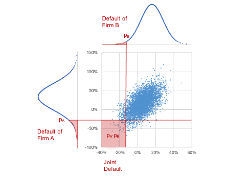
Without going into more details of the Merton model, we move on to one of its more interesting aspects, namely that joint defaults are the result of dependency on firm values in the economy. If we model firm values as variables of a multivariate normal distribution, we can visually represent default and joint default for two firms like this:

We see that default events are both univariate left tail events as well as joint left tail events. And that the joint default probability is driven by the correlation between firm values, assumed to be 60% in the scatter plot above.

Moody’s KMV Company uses a methodology that allows calculating default-implied asset correlation between firms. The tables below show results for sectors and ratings. 

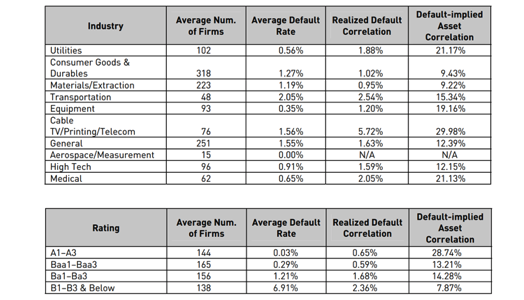
The Cable TV/Telecom sector has the largest default-implied correlation because of the unprecedented clustering of telecom defaults in 2001 and 2002. Default-implied correlations seem to increase with better ratings.

Various refinements of the Merton model have been proposed and studied. For the purposes of our discussion, we will modify the dependency assumption of the Merton model in a very specific manner.

Copula Theory, Gaussian And Clayton Copulas

Many financial market practitioners, as well as researchers, equate ‘dependency’ with ‘correlation’. This is problematic for several reasons; the richest and most general model of dependency can be found in Copula theory. In a nutshell, a Copula is a valid probability distribution with the following additional properties:

• The Copula is the distribution that connects the distributions of the input variables (the marginal distributions) so that the joint probability distribution of the input variables is generated. It can also be shown that valid joint distributions can almost always be decomposed into marginal distributions and a unique Copula.

For example, a multivariate normal distribution can be decomposed into marginal distributions that are normal and a Gaussian copula defined by a correlation matrix.

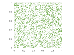
One side-effect of Copula theory is that dependency can no longer be visualised in return scatterplots because they do not show pure dependency, but the combined result of marginal distributions and the copula. Copulas can be visualized by ‘standardizing’ the marginal distributions. This is typically done by transforming observed returns into probabilities with the help of the inverse cumulative distribution functions. The resulting scatter plot is called unit space. Independent variables cover unit space evenly, as seen in the chart below.

The next charts below show normally distributed variables. To the left, we see returns correlated by 80%, and to the right, we see the corresponding Gaussian copula in unit space…

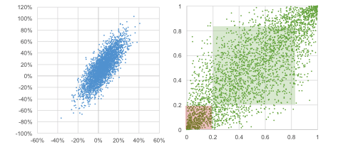
The points generated by a Gaussian copula do not evenly cover unit space anymore. When analysing the properties of the Gaussian copula, one quickly realises that the dependency pattern mainly arises from the dependency of the variables in the middle (green area). In the tails (red area), observations are spread out evenly, similar to the independent case shown above. This is not a coincidence: analytically, it demonstrates that tail dependency of a Gaussian copula converges to zero.

Therefore, it should be clear that a Gaussian dependency structure is not an adequate model for far-left tail events, like defaults. This became apparent during the Financial Crisis in the context of the pricing of CDO tranches, in which default dependency between tranches is the relevant pricing factor due to the waterfall structure of this debt vehicle.

An interesting Copula model for left tail events is the Clayton Copula, defined as…

C_Clayton(u,v) = (u^-θ + v^-θ – 1)^-1/θ

With u, v being probabilities (0,1) from two marginal distributions and a ‘tail dependency’ parameter θ defined across (0, ∞). In unit space, the dependency from a Clayton Copula looks like this:

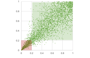
The important aspect of Clayton Copulas is that they define dependency based on correlations in left tails (red area). Any points outside the left tail (green area) are very much independent; this makes Clayton Copulas a valuable model in credit risk applications, stress testing, and extreme scenario analysis in general.

Simulating Dependent Joint Defaults

The charts below are based on a simulation of joint default probabilities from three models of default dependency: independence, Gaussian Copula and Clayton Copula. The main result (red shaded line) is that correlated defaults significantly increase joint default probability (an increase from 1.54% to 3.81%), with more realistic tail dependency models - as in the case of a Clayton Copula -further increasing joint default probability (4.75%).

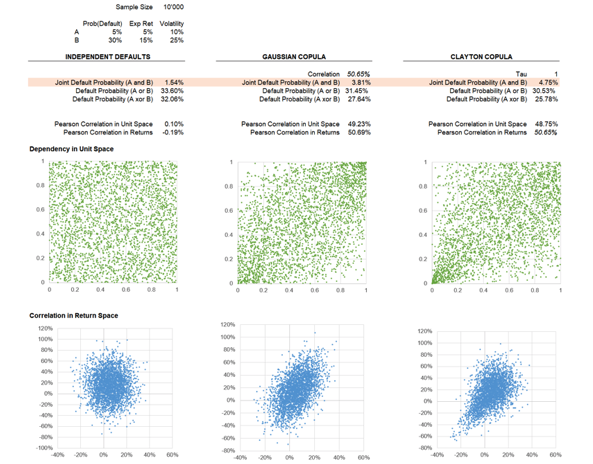
Note that we did not calibrate the Clayton dependency parameter to empirical default data; we set a tau value and derived the Gaussian Copula exhibiting the same average correlation in returns (50.65%). The returns can be interpreted as firm assets values, and as a one-factor model of default – correlated factor exposure imply firm-specific betas to the underlying credit risk factor.

Our simulations imply an approximatively 50% asset correlation for a stress scenario, a result consistent with Moody’s default-implied correlation for the Cable TV/Telecom sector of around 30% in the years of clustered defaults 2001 and 2002.

The simulation spreadsheet makes use of built-in Excel functions only and is available on request.

Implications for Portfolio Default Risk Management

In many practical applications – internal risk reporting, client reporting, fund factsheets and similar – portfolio-level default risk is calculated as the asset-weighted portfolio constituent ratings. This calculation assumes that joint default probabilities are either zero or small enough to ignore their impact on portfolio risk. While this might be adequate in normal times, it will fail in regimes with clustered defaults or major changes in default risk, due to, for example, clustered downgrades.

Additionally, factors affecting firm defaults can be expected to exhibit larger downside dependency relative to a) standard model assumption – especially the Gaussian Copula – and b) average correlations taking into account the dependency in ‘normal’ market regimes only. This can lead to an underestimation of expected losses, especially in turbulent times.

With the volatility of credit risk expected to increase, investors should utilise credit risk analytics that can adequately assess the impact of credit tail events in a forward-looking manner.

To some degree, this is already standard practice in the management of bank balance sheets. However, in a world where increasing corporate and sovereign debt forces investors to raise credit exposures due to low yields, a proper understanding of credit risk in the context of investment portfolios is becoming an essential risk management skill – also in buy-side investment management.

In a world of increasing debt, it's important to have a firm grip on default dependancy and how it could impact your portfolio risk management. If you need assistance understanding more about this topic or would like access to our specialist course, please contact us today. 

Our courses are taught by world-leading financial experts and provide the latest knowledge to boost your career or company performance. 

Related Courses

Sources:

Çelik/Demirtaş/Isaksson (2020), “Corporate Bond Market Trends, Emerging Risks and Monetary Policy”, OECD Capital Market Series, Paris